One of the features in Polars is LazyFrame. Polars is fast as is, and LazyFrame gives you even more optimizations.
But you may wonder, “How is it different from the typical DataFrame or EagerFrame?” or “What is LazyFrame in the first place”?
What is LazyFrame in Polars
In order to understand LazyFrame, it’s good to start with learning the difference between eager evaluation and lazy evaluation.
Eager evaluation is where an expression is evaluated immediately when it’s called. So when you read a csv file for example and assign that to a variable called df, then the data gets processed or materialized immediately right when your code evaluates that line of code. And this is what DataFrame or EagerFrame uses in Polars.
Lazy evaluation is a technique to delay the evaluation of an expression until it’s actually needed. LazyFrame is simply a DataFrame that utilizes this lazy evaluation. For instance, if you’re reading a csv file with 3 columns and applying “select()” to select only 1 column, with lazy evaluation, that “select” portion gets pushed to when you read the csv file. That means you actually only process data with that 1 column. You can see how lazy evaluation makes your operations more efficient especially when you work with large datasets.
LazyFrame in Polars has several optimizations such as predicate pushdown and projection pushdown. You can check out the full list on Polars documentation.
One limitation of LazyFrame is that not all expressions and methods are available. For example, pivot() is availabe in DataFrame, but not in LazyFrame because it needs to know the schema which requires materializing the whole dataset.
Essentially, LazyFrame is more an efficient way of working with a dataset than using DataFrame. If you replace your DataFrame with LazyFrame in your Polars code, it may get a faster execution time.
LazyFrame vs DataFrame – Performance Comparison
Now the question is “How fast is a LazyFrame compared to a DataFrame?”. The answer is, it depends. It depends on your data size as well as the complexity of your transformations.
I did a performance test anyways though. I wanted to do a generic comparison to see how much of an impact LazyFrame would have on the random transformations I came up with.
Setup
I used a 16-inch, Apple M1 Max MacBook Pro 2021 with 64GB RAM and 1TB SSD. The total number of cores is 10 (8 performance and 2 efficiency). I also use macOS Ventura at the time of writing this post.
(You might’ve noticed If you’d read my other post comparing Pandas vs Polars, but yes, I upgraded my laptop from my old 2015 MacBook Pro!)
Data
I used “2021 Yellow Taxi Trip Data” from data.gov. Here’s the link to the dataset.
It contains 30,904,072 rows and 18 columns. The size of the dataset is 3GB. Not sure if we can call it a large dataset, but it’s not small.
Code
I created 4 functions for transformations to test, and a few other utility functions. You can find the full code in my GitHub repo.
def select_n_filter_columns(df):
    return (
        df
        .select(pl.col('VendorID', 'tpep_pickup_datetime', 'total_amount', 'tolls_amount', 'payment_type', 'tip_amount', 'fare_amount', 'PULocationID'))
        .filter(pl.col('total_amount') > 100)
    )
def some_groupby_agg(df):
    return (
        df
        .groupby('VendorID', 'payment_type', 'PULocationID')
        .agg(
            pl.col('tip_amount').mean().alias('avg_tip_amount')
        )
    )
def some_window_func(df):
    return (
        df
        .select(
            pl.col('VendorID'),
            pl.col('payment_type'),
            pl.col('tpep_pickup_datetime'),
            pl.col('PULocationID'),
            pl.col('tip_amount'),
            pl.col('fare_amount').mean().over('payment_type').alias('mean_fare_amt_per_payment_type'),
        )
        .with_columns(
            pl.col('mean_fare_amt_per_payment_type').rank('dense', descending=True).over('VendorID').alias('dense_rank')
        )
    )
def join_on_a_few_column(df):
    unique_vendor_id_df = df.select('VendorID', 'payment_type', 'PULocationID').unique()
    return (
        df
        .join(unique_vendor_id_df, on=['VendorID', 'payment_type', 'PULocationID'], how='left')
    )
def write_to_csv(df):
    output_file_name = 'output.csv'
    if type(df) == pl.LazyFrame:
        df.collect().write_csv(output_file_name)
        return

    return df.write_csv(output_file_name)
Result
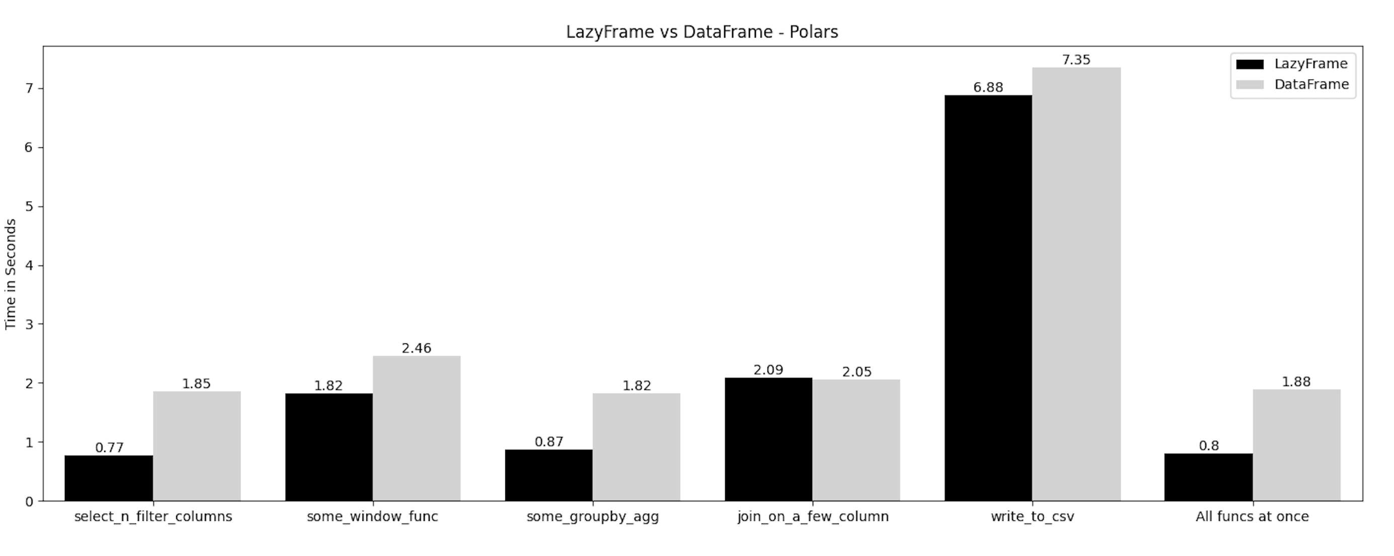
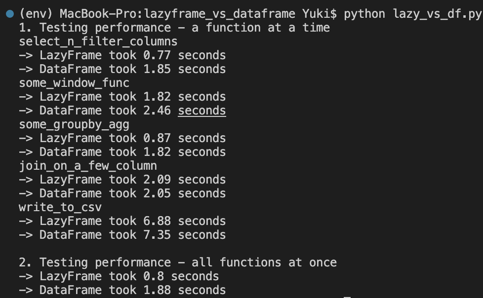
The result is not necessarily what I expected. I expected more performance boost for LazyFrame.
It’s interesting the performance for the join operation is pretty much the same between LazyFrame and DataFrame. I wonder why LazyFrame is not able to take advantage of its optimizations on this join.
The overall performance gain is around ~2.5x. Perhaps it’s sufficient improvement given the size of the dataset. LazyFrame is indeed faster and the difference may be bigger when you work larger dataset.
Now that I look at this result, writing data out to a csv file without any transformation is not even a comparison. I’m just doing the same thing in two different ways. No wonder they show pretty much the same result.
Raw output:

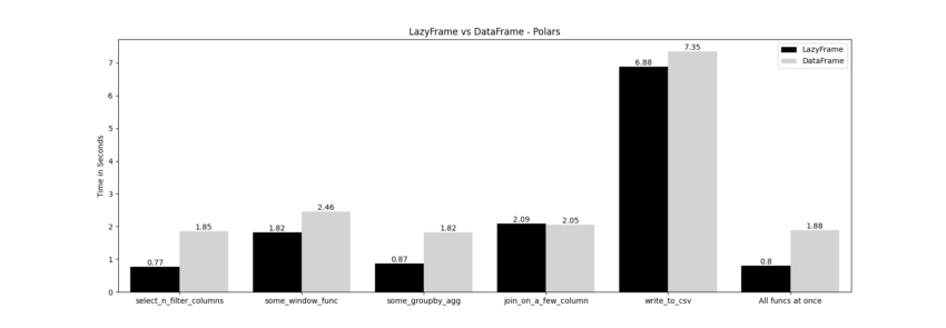
Visualization:

Limitations
The choice of the dataset and kind of transformations I did are super subjective. There is no logical reason for why I did what I did in a certain way. The same goes for the order I applied functions at once in a chain (“All func at once” test).
For the join operation, I join a unique combination of a few columns because when I did a many-to-many join without getting unique values, the code didn’t run that it just killed the process automatically. So I needed to make sure to do a many-to-one join that the operation was feasible.
Another thing is that even though I’m pretty comfortable working with Polars at this point, but my code may or may not be the most optimized format.
Lastly, I didn’t check anything for the load on memory & CPU. There may or may not have been significant difference.
Summary
Hope this blog post gives you an idea of what LazyFrame is in Polars and its performance gain compared to DataFrame. Polars is already fast without LazyFrame, but it’s faster when you use LazyFrame. Maybe I try using a bigger dataset next time to see what difference we can observe.
