

Introduction
One advantage Polars brings is its ability to evaluate queries lazily (lazy mode) instead of executing code immediately (eager mode). This allows the Polars engine to apply optimizations to your query. Polars uses dataframes for eager evaluation and lazyframes for lazy evaluation.
In this post, we’ll cover how to inspect and optimize query plans in Python Polars. You can find the code in this GitHub repo.
Inspect Query Plans
There are two methods you can use to inspect query plans.
- explain
- show_graph
The .explain() method shows the query plan in a text format. On the other hand, the .show_graph() method visualizes the query plan. You’ll need to install the GraphViz package and add it to your PATH for using the .show_graph() method.
Here are the code examples for using those methods.
The .explain() method
import polars as pl

print(
    pl.scan_csv('pokemon.csv')
    .filter(pl.col('Type 1')=='Grass')
    .with_columns(pl.col('HP').max().alias('Max HP'))
    .filter(pl.col('HP')>300)
    .select('Name', 'Type 1', 'HP', 'Max HP')
    .explain()
)
'''
FILTER [(col("HP")) > (300)] FROM
   WITH_COLUMNS:
   [col("HP").max().alias("Max HP")]
    Csv SCAN [pokemon.csv]
    PROJECT 3/13 COLUMNS
    SELECTION: [(col("Type 1")) == (String(Grass))]
'''
It returns the optimized query plan by default. If you want to show a non-optimized query plan, you’ll need to set the optimized parameter to False:
print(
    pl.scan_csv('pokemon.csv')
    .filter(pl.col('Type 1')=='Grass')
    .with_columns(pl.col('HP').max().alias('Max HP'))
    .filter(pl.col('HP')>300)
    .select('Name', 'Type 1', 'HP', 'Max HP')
    .explain(optimized=False)
)
'''
SELECT [col("Name"), col("Type 1"), col("HP"), col("Max HP")] FROM
  FILTER [(col("HP")) > (300)] FROM
     WITH_COLUMNS:
     [col("HP").max().alias("Max HP")]
      FILTER [(col("Type 1")) == (String(Grass))] FROM
        Csv SCAN [pokemon.csv]
        PROJECT */13 COLUMNS
'''
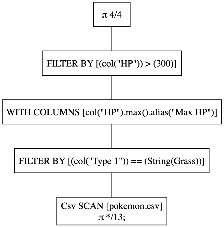
If you look at the line that says “Csv SCAN [pokemon.csv]” and below, this non-optimized query plan doesn’t include filtering and column selection at the scan level. Whereas, if you look at the optimized query plan above, there are only 3 columns selected and data is filtered where the “Type 1” column equals “Grass” at the scan level.
As you can see, using a lazyframe benefits from optimizations that are not available in dataframes.
The .show_graph() method
Let’s run the same queries using the .show_graph() method.
(
    pl.scan_csv('pokemon.csv')
    .filter(pl.col('Type 1')=='Grass')
    .with_columns(pl.col('HP').max().alias('Max HP'))
    .filter(pl.col('HP')>300)
    .select('Name', 'Type 1', 'HP', 'Max HP')
    .show_graph()
)
The output looks like the following:

We can see the same kinds of optimizations in the graph as we saw with the .explain() method.
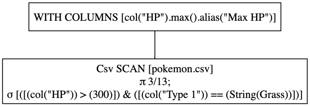
Now let’s run the non-optimized query:
(
    pl.scan_csv('pokemon.csv')
    .filter(pl.col('Type 1')=='Grass')
    .with_columns(pl.col('HP').max().alias('Max HP'))
    .filter(pl.col('HP')>300)
    .select('Name', 'Type 1', 'HP', 'Max HP')
    .show_graph(optimized=False)
)
The output looks like the following:
As you can see, filtering and column selection are not happening at the scan level.
Optimize Query Plans
If you look at the code carefully, you notice that even in the optimized query plan, there is one filter that’s not pushed to the scan level. Which is a filter on the “HP” column where we only keep rows whose HR is greater than 300.
Polars tries its best to find inefficiencies in your query, however, sometimes you may find cases like this. That’s why the .explain() and .show_graph() methods are very useful in finding things that could be optimized.
Now, what I’m going to show is a very simple thing, which is to move up this filtering logic earlier in the query:
(
    pl.scan_csv('pokemon.csv')
    .filter(pl.col('Type 1')=='Grass')
    .filter(pl.col('HP')>300)
    .with_columns(pl.col('HP').max().alias('Max HP'))
    .select('Name', 'Type 1', 'HP', 'Max HP')
    .show_graph()
)
And this is the output:
Boom! Now we see the filtering logic pushed to the scan level. We successfully optimized the query!
Check the Execution Time for Each Operation in your Query
Aside from the two methods introduced above, there is the .profile() method that shows a table containing the information on how long it took for Polars to execute each operation. This is useful when trying to identify the exact operation that might needs some tweaking.
(
    pl.scan_csv('pokemon.csv')
    .filter(pl.col('Type 1')=='Grass')
    .filter(pl.col('HP')>300)
    .with_columns(pl.col('HP').max().alias('Max HP'))
    .select('Name', 'Type 1', 'HP', 'Max HP')
    .profile()
)
'''
(shape: (0, 4)
 ┌──────┬────────┬─────┬────────┐
 │ Name ┆ Type 1 ┆ HP  ┆ Max HP │
 │ ---  ┆ ---    ┆ --- ┆ ---    │
 │ str  ┆ str    ┆ i64 ┆ i64    │
 ╞══════╪════════╪═════╪════════╡
 └──────┴────────┴─────┴────────┘,
 shape: (3, 3)
 ┌─────────────────────────────┬───────┬──────┐
 │ node                        ┆ start ┆ end  │
 │ ---                         ┆ ---   ┆ ---  │
 │ str                         ┆ u64   ┆ u64  │
 ╞═════════════════════════════╪═══════╪══════╡
 │ optimization                ┆ 0     ┆ 51   │
 │ csv(pokemon.csv, predicate) ┆ 51    ┆ 1825 │
 │ with_column(Max HP)         ┆ 1864  ┆ 2041 │
 └─────────────────────────────┴───────┴──────┘)
'''
The .profile() method returns a tuple containing a materialized dataframe and a table with profiling information. Note that in our specific example, there are no rows returned because the filters in the query filtered out all the rows.
Summary
Although Polars is already fast and efficient, it’s good to know how to inspect and optimize your queries in Polars!
P.S. I include tips like this in Polars Cookbook. If you haven’t, make sure to check it out on GitHub and Amazon!